terça-feira, 26 de maio de 2020

Datação por carbono é recalibrada e deve mudar idade dos fósseis

24/05/2020 às 14:00

2 min de leitura

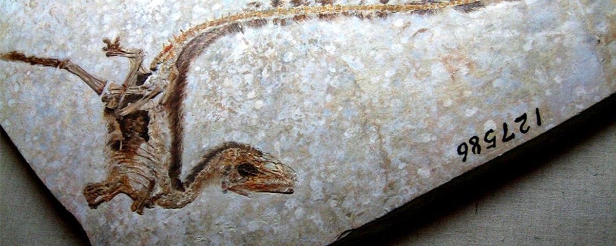
Imagem: The Nanjing Institute/Divulgação

Desde sua criação, em 1960, a datação por radiocarbono é usada para determinar a idade de qualquer coisa, de livros e esqueletos a múmias e marfim traficado. Agora, esse sistema será recalibrado com a inclusão de milhares de dados obtidos desde sua última versão, de 2013.

“Uma nova curva de calibração é de importância fundamental para a compreensão da pré-história e da cronologia dos hominídeos", diz o cronologista arqueológico e diretor da Unidade de Acelerador de Radiocarbono de Oxford, Tom Higham.

Esse ajuste está sendo feito não apenas para melhor entender o passado, mas para compensar o presente, que hoje despeja bilhões de toneladas de carbono no meio ambiente. A queima de combustíveis fósseis e os testes de bombas nucleares mudaram radicalmente a quantidade de carbono-14 no ar.
A datação por radiocarbono pode dizer quando o homem moderno surgiu.

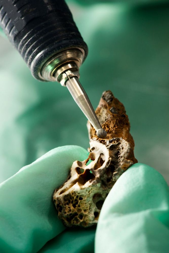
A datação por radiocarbono pode dizer quando o homem moderno surgiu.Fonte: Science Photos/Reprodução

Poluição altera o equilíbrio

Quase 99% de todo o carbono da Terra está na forma de seu isótopo com 12 nêutrons em seu núcleo; o carbono-12 é a forma mais estável do elemento. A técnica de datação por radiocarbono mede a presença de um isótopo instável e por isso, muito mais raro: o carbono-14 que, na natureza, é produzido a uma taxa constante na atmosfera superior da Terra.
Quando uma planta ou um animal morre, para de absorver esse isótopo, e o que foi acumulado começa a decair. Medir a quantidade restante fornece uma estimativa de há quanto tempo algo morreu.
O problema é que a humanidade, principalmente nas últimas décadas, tem lançado na atmosfera o carbono de combustíveis fósseis, que não têm mais uma quantidade mensurável de carbono-14. O resultado é que bilhões de toneladas de carbono-12 artificialmente postas na balança estão arruinando a proporção constante entre os dois isótopos.

Árvores guardam um calendário confiável

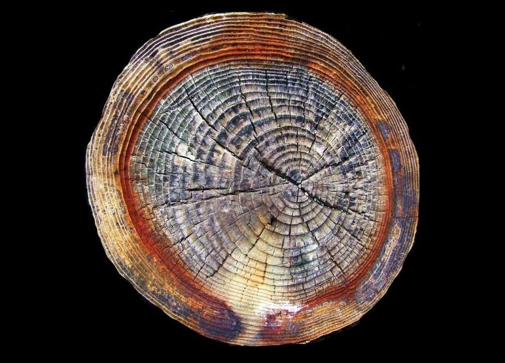
Os anéis das árvores ajudam a calibrar a curva de datação por radiocarbono.Fonte: Flickr/Tina Negus/Reprodução
Para produzir uma curva que possa ser usada para relacionar anos do calendário com os determinados pelo radiocarbono, é necessária uma sequência de amostras com data seguramente conhecida, como os anéis no tronco de uma árvore. Os cientistas usam esse método combinado com informações de sedimentos de lagos e oceanos, corais e estalagmites para calibrar o sistema.

Desde 1998 é usada o sistema IntCal (IntCal98), que já sofreu três atualizações: em 2004, 2009 e 2013. Agora, está sendo lançada a versão 2020, com as novas curvas para os hemisfério Norte (IntCal20) e sul (SHCal20) e mais para amostras marinhas (MarineCal20).

Mais velho, mais jovem

A IntCal20 é baseada em 12.904 pontos de dados, quase o dobro do tamanho do conjunto de dados de 2013. Isso tornou, por exemplo, mais acurada a datação de um maxilar do Homo sapiens encontrado em 2002 na Pe?tera cu Oase (Ou a Caverna com Ossos), na Romênia.
A mandíbula do Osase 1, o homem moderno mais antigo já encontrado.

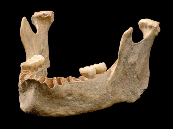
A mandíbula do Osase 1, o homem moderno mais antigo já encontrado.Fonte: FU Qiaomei/Phys.org/Reprodução

Ali foram escavados os restos mais antigos de humanos modernos (entre 35 e 40 milhares de anos). A idade do exemplar denominado Oase 1 foi reavaliada pela nova curva; ele é centenas de anos mais velho do que se pensava. Análises genéticas ainda revelaram que ele tinha um ancestral neandertal, distante de quatro a seis gerações.

“Isso significa que, quanto mais antigo o Oase 1 é, mais neandertais andavam pela Europa”, explica Higham. Em contrapartida, o adolescente cujos fósseis foram desenterrados na Sibéria viveu mil anos à frente do que se pensava e isso, segundo o cronólogo, muda a história da chegada dos humanos modernos na Sibéria.a

sábado, 23 de maio de 2020

Este escorpião foi uma das primeiras formas de vida a andar na Terra

Damares Alves

19/01/2020

Um fóssil do Parioscorpio venator , um escorpião de 437 milhões de anos que se assemelha a espécies modernas, foi um das primeiras formas de vida a andar na Terra, (Wendruff et al., Scientific Reports, 2020)

Há quase 500 milhões de anos atrás artrópodes blindados com corpos segmentados e membros articulados, moluscos sem casca e organismos vacilantes e irreconhecíveis caminhavam pela Terra. Dentre essas criaturas estava um escorpião que tinha a capacidade de respirar tanto nas águas dos oceanos antigos quanto em terra. Agora, paleontólogos conseguiram identificar um fóssil deste escorpião pré-histórico.

Uma das primeiras formas de vida a andar na Terra

Um artigo publicado na revista Scientific Reports descreve o pequeno artrópode 2,5 centímetros que viveu durante o período geológico siluriano de 443 a 416 milhões de anos atrás. O Parioscorpio venator, como foi batizado o pequeno predador, empurra a data do primeiro escorpião conhecido em até três milhões de anos. Além disso, ele é a evidência mais antiga de qualquer criatura com aparelho respiratório capaz de andar na terra.

Dois espécimes fósseis de Parioscorpio venator, desenterrados em Wisconsin. Este escorpião foi uma das primeiras formas de vida mais antiga a andar na Terra. (Wendruff et al., Scientific Reports, 2020)

Segundo o estudo, o que permitia que esses pequenos predadores pudessem respirar tanto na terra quanto no mar, eram seu ‘seios pulmo-pericárdicos’.

O sistema respiratório e circulatório do escorpião são quase idênticos aos escorpiões modernos que conhecemos, mas operavam de forma semelhante ao de um caranguejo-ferradura, que vive principalmente na água, mas que é capaz de fazer incursões curtas na terra.

Um fóssil de Parioscorpio venator (a) comparado a uma imagem microscópica de Centruroides exilicauda (b) e Hadogenes troglodytes (c), ambos escorpiões modernos. "bl" significa pulmões de livros, uma estrutura respiratória, e "pc" representa pericárdio, uma estrutura que envolve o coração. As barras de escala são de 1 milímetro para aeb e 1 centímetro para c. (Wendruff et al., Scientific Reports, 2020) — Um fóssil de Parioscorpio venator (a) comparado a uma imagem microscópica de Centruroides exilicauda (b) e Hadogenes troglodytes (c), ambos escorpiões modernos. “bl” significa pulmões de livros, uma estrutura respiratória, e “pc” representa pericárdio, uma estrutura que envolve o coração. As barras de escala são de 1 milímetro para aeb e 1 centímetro para c. (Wendruff et al., Scientific Reports, 2020)

O antigo escorpião tinha capacidade de respirar fora da água, mas isso significa que ele o fazia?

O fóssil do Parioscorpio venator foi encontrado em um ambiente de águas rasas e provavelmente viveu no mar, mas seu sistema respiratório os permitia viver fora da água. Os ‘seios pulmo-pericárdios’ conectavam os órgãos respiratórios da criatura com o seu sistema circulatório, assim como os escorpiões que caçam pela Terra atualmente, entretanto este é um fóssil muito antigo e não foram encontradas evidências de pulmões ou guelras, portanto seria precipitado afirmar com certeza que esses escorpiões viveram na terra ou no mar. É apenas uma possibilidade, e ela entusiasmante.

Um fóssil do Parioscorpio venator , um escorpião de 437 milhões de anos que se assemelha a espécies modernas. b mostra sua pinça esquerda; c mostra seus olhos compostos; d e e mostram suas estruturas respiratórias e circulatórias; f mostra o final de sua cauda. (Wendruff et al., Scientific Reports, 2020)

Há 440 milhões de anos uma outra forma de vida já dominava a Terra

Embora o escorpião seja o animal mais antigo a emergir dos mares para a terra até agora, quando ele chegou lá estava longe de estar sozinho, pois uma outra forma já havia se estabelecido nos solos antigos: Os Tortotubus.

Filamento principal de T. protuberans com ramos primários e ramos secundários nascentes. (verisimilus / CC BY 3.0)

Um estudo publicado no Botanical Journal da Linnean Society, demonstrou como os fungos fossilizados, chamados Tortotubus, viviam há cerca de 440 milhões de anos atrás.

FONTES / Smithsonian / Science Daily

Entenda como são feitas as datações de fósseis

Damares Alves

22/01/2020

Entenda como são feitas as datações de fósseis

Compartilhe Tweet

Fósseis não vêm com certidão de nascimento, mas ainda assim eles trazem muitas informações que podem nos ajudar a reconstruir sua trajetória. Muitas pessoas ainda tem dúvidas sobre como são feitas as datações e se elas são concisas, por isso é importante esclarecer como como os cientistas determinam as idades destas estruturas petrificadas. Existem dois métodos principais usados para fazer as datações de fósseis e rochas, são eles a datação relativa e a datação absoluta.

Como são feitas as datação relativas de fósseis

A datação relativa é usada há muito tempo, antes do surgimento dos métodos mais precisos desenvolvidos há algumas décadas. Consiste em se observar a posição das rochas sedimentares. Por exemplo; se uma camada de sedimentos foi datada anteriormente para aproximadamente 200 milhões de anos, então sabemos que o fóssil lá encontrado também tem cerca de 200 milhões de anos. Esse método não oferece uma data numérica, mas nos ajuda a entender em qual período a criatura descoberta viveu.

Até hoje os métodos de relativa são amplamente utilizados, devido a sua praticidade e baixo custo. Um deles consiste em verificar a camada de sedimentos em que os fósseis foram encontrados. (Imagem: Damares / Redação SoCientífica)

Até os dias atuais os métodos de datações relativas são usados como uma primeira abordagem para datar fósseis antes de atribuir uma idade numérica ou absoluta.

A datação absoluta

A datação absoluta determina a idade precisa de uma rocha ou fóssil através de métodos de datação radiométrica usando minerais radioativos que são encontrados em rochas e fósseis, eles servem como um relógio biológico. Muitas vezes, as camadas de rochas vulcânicas – rochas vulcânicas normalmente contêm minerais naturalmente radioativos – acima e abaixo das camadas que contêm os fósseis podem ser datadas para fornecer um intervalo de datas para as rochas onde estão os fósseis.

Um feldspato mineral naturalmente radioativo, visto ao microscópio. Minerais radioativos funcionam como relógios naturais que ajudam a fazer as datações de fósseis e rochas. (Erin DiMaggio, Penn State University)

Usando técnicas baseadas no decaimento radioativo de isótopos podemos chegar a idade de um fóssil. Medindo-se a razão entre a quantidade do isótopo original (isótopo pai) e a quantidade dos isótopos em que que ele se divide, (isótopos filhos) a idade do fóssil pode então ser determinada.

A taxa desse decaimento radioativo é chamada meias-vidas. Se um isótopo radioativo tem uma meia-vida de 5.000 anos, isso significa que, depois de 5.000 anos, exatamente metade dele terá decaído do isótopo pai para os isótopos filhos. Depois de outros 5.000 anos, metade do isótopo pai restante terá decaído.

Carbono-14 e potássio-40

Embora as pessoas estejam muito mais familiarizadas com a datação por carbono, ela raramente é aplicável aos fósseis. Isso por que o isótopo radioativo do carbono usado na datação por carbono, tem uma meia-vida de 5730 anos, por isso decai muito rapidamente. Por isso a datação por carbono só pode ser usada para datar fósseis com menos de 50.000 anos.

Já o potássio-40, tem meia vida de 1,25 bilhão de anos e é comum em rochas e minerais. Isso o torna ideal para datar rochas e fósseis muito mais antigos. Como é o exemplo de um escorpião de 443 milhões de anos, que é considerado o animal terrestre mais antigo já descoberto.

Outros métodos de datações de fósseis

Atualmente os cientistas já tem uma grande quantidade de ferramentas à sua disposição, mas, ainda assim, algumas rochas e fósseis são difíceis de serem datadas. As inovações nos métodos de datação existentes estão eliminando essas barreiras. Por exemplo, as revisões de um método chamado ressonância de rotação eletrônica permitem que os cientistas datem fósseis raros, porque podem datar diretamente o fóssil sem danificar visivelmente a amostra.

sexta-feira, 22 de maio de 2020

Ancient human genomes shed new light on East Asia's history

14 May 2020

First large-scale ancient genome analyses from China chart migrations of early farmers.

Ewen Callaway

Whole skeleton of Qihe 2, a ~8,400-year-old individual from Qihe cave, Fujian, China. — An 8,400-year-old skeleton from the Qihe cave archaeological site in Fujian, China.Credit: Xiujie Wu/Institute of Vertebrate Paleontology and Paleoanthropology

A genômica antiga está começando a desvendar a história do leste da Ásia. Os primeiros estudos em larga escala de genomas humanos antigos da região sugerem que muitos de seus habitantes descendem de duas populações outrora distintas que começaram a se misturar após o desenvolvimento da agricultura, cerca de 10.000 anos atrás.

Os estudos também revelam conexões entre humanos antigos que se estendem do sul da China ao Pacífico Sul, e um elo entre habitantes costeiros que poderia oferecer pistas sobre como os humanos se estabeleceram no leste da Ásia.

Os resultados são de um estudo de 14 de maio na Science que analisou os genomas de duas dúzias de chineses antigos1 e uma pré-impressão de março que analisou quase 200 genomas antigos de todo o leste asiático2.
Os asiáticos orientais contemporâneos descendem, em geral, de humanos que deixaram a África entre 50.000 e 100.000 anos atrás.

Mas os pesquisadores sabem pouco sobre as antigas mudanças populacionais que moldaram os genomas dos 1,7 bilhão de habitantes atuais da região. Apenas um punhado de genomas humanos antigos do Leste da Ásia foi publicado, e não está claro como eventos importantes, como a disseminação da agricultura - que alterou drasticamente a composição genética dos eurasianos ocidentais - afetaram essa parte do mundo.

Uma equipe liderada por Qiaomei Fu, geneticista populacional do Instituto de Paleontologia e Paleoantropologia de Vertebrados em Pequim, analisou os genomas de 24 indivíduos que viviam no leste da Ásia, incluindo o que é hoje a China, entre 9.500 e 300 anos atrás. A maioria dos genomas veio de sítios arqueológicos na Bacia do Rio Amarelo, no nordeste da China, ou a mais de 1.000 quilômetros de distância, na província de Fujian, no sudeste da China.

North–South divide

Durante o período neolítico inicial, cerca de 10.000 a 6.000 anos atrás, as pessoas dessas duas regiões geográficas eram geneticamente distintas, concluiu a equipe de Fu. Mas, com o tempo, começaram a se misturar: os chineses contemporâneos traçam grande parte de seus ancestrais aos grupos do norte, mas também estão relacionados ao antigo povo Fujian em graus variados (os do sul da China tendem a ser os mais próximos). A equipe de Fu não sabe exatamente quando os dois grupos começaram a se cruzar, mas viu sinais de que a assinatura genética do norte havia começado a se espalhar para o sudeste da China na época do final do neolítico de 5.000 a 4.000 anos atrás.

This suggests that farming in East Asia could have spread through mixing of farmers and hunter-gatherers, says Ling Qin, an archaeologist at Peking University in Beijing. That’s different from what ancient-genome studies have found in western Eurasia, where farmers with Middle Eastern ancestry largely replaced hunter-gatherers in Europe³.
Farmers in the Yellow River Basin also moved west. A team led by David Reich, a population geneticist at Harvard Medical School in Boston, Massachusetts, who is a co-author of Fu’s study, analysed the genomes of 20 5,000-year-old individuals from this region and found connections with contemporary Tibetans. Their results are part of a study of 191 ancient individuals from East Asia that was posted to the bioRxiv preprint server on 25 March.

Distant relatives

The studies also revealed some surprising long-distance connections. Neolithic people who lived near China’s coast, whether in the northeast or southeast, shared some ancestry with ancient individuals from coastal sites in southeast Asia and Japan. “That means the entire coast of East Asia is a really important place for people to migrate,” says Fu. Reich and his team found a similar connection, which they say could be evidence that modern humans first settled in East Asia along a coastal route.

Ancestry from southeastern China stretched even farther afield. Neolithic individuals from Fujian and islands in the Taiwan Strait were closely related to ancient islanders from Vanuatu in remote Oceania, Fu’s team found. Previous ancient-genome studies had recorded the spread of this ancestry from East Asia to Oceania⁴, and Fu’s study suggests that this group originated in southern China.

This conclusion makes sense, says Matthew Spriggs, an archaeologist at Australian National University in Canberra. Archaeological and genetic evidence has linked the South Pacific migration to ancient humans in Taiwan, whose Neolithic inhabitants probably came from southern parts of the mainland. “I am very pleased to see this paper,” he says of Fu’s study.

Qin says that the ancient southern Chinese people in Fu’s study lived in an isolated pocket that might not be representative of the wider area. A priority should be sequencing DNA from early farmers from the Yangtze River Basin in southern China, a centre for rice domestication and a potential source of other migrations, she adds.

The studies give researchers hope that ancient genomics will help them delve even deeper into East Asia’s early history. Pontus Skoglund, a population geneticist at the Francis Crick Institute in London, would love to know whether the first Homo sapiens to settle in the region interbred with Denisovans, an extinct group of hominins. “I think one of the most exciting open big questions of the region relates to the pre-Neolithic settlement — who were the earliest modern humans in the region?” adds Martin Sikora, a geneticist at the University of Copenhagen.

doi: 10.1038/d41586-020-01456-9

References

1.
M. A. Yang et al. Science https://doi.org/10.1126/science.aba0909 (2020).

Phenotypic plasticity as a long-term memory easing readaptations to ancestral environments

Plasticidade fenotípica como memória de longo prazo, facilitando a readaptação a ambientes ancestrais

See all authors and affiliations

Science Advances 22 May 2020:
Vol. 6, no. 21, eaba3388
DOI: 10.1126/sciadv.aba3388

Abstract

Plasticidade fenotípica refere-se a alterações fenotípicas induzidas pelo ambiente sem mutação e está presente em todos os organismos. O papel da plasticidade fenotípica nas adaptações orgânicas para novos ambientes atraiu muita atenção, mas seu papel nas readaptações para ambientes ancestrais é pouco estudado. Para abordar essa questão, usamos a abordagem de transplante recíproco para investigar os transcriptomas multissetoriais de galinhas adaptadas ao platô tibetano e à planície adjacente. Embora muitas mudanças transcriptômicas genéticas tenham ocorrido na adaptação direta às terras altas, as mudanças plásticas transformam amplamente os transcriptomas no estado preferido quando as galinhas tibetanas são trazidas de volta às terras baixas. A mesma tendência se aplica à eclodibilidade dos ovos, um componente essencial da aptidão dos frangos. Essas descobertas, juntamente com padrões altamente semelhantes em experimentos comparáveis de guppies e Escherichia coli, demonstram que os organismos geralmente “lembram” seus ambientes ancestrais via plasticidade fenotípica e revelam um mecanismo pelo qual a experiência passada afeta a evolução futura.

INTRODUCTION

Organismal adaptation to a new environment often consists of two steps. The first step involves plastic phenotypic changes without mutational input, while the second step involves genetic phenotypic changes resulting from the fixations of mutations advantageous in the new environment. It is important to clarify the relationship between these two steps of phenotypic changes for a comprehensive understanding of environmental adaptation. In particular, discussions have focused on the question of whether plastic changes serve as stepping-stones to genetic adaptations (1–6). While earlier studies on a small number of morphological, physiological, or behavioral traits did not reveal a general trend, recent experimental evolution studies have shown that plastic gene expression changes tend to be reversed rather than reinforced by subsequent genetic changes, casting doubts on the contribution of phenotypic plasticity to environmental adaptations (7–12). Nevertheless, because these recent studies examined organismal adaptations to novel environments only, it remains possible that the role of phenotypic plasticity is much greater in readaptations to ancestral environments. Using gene expression levels as focal traits, we explore this possibility by investigating cases of domestication, experimental evolution, and/or natural evolution of animals and bacteria. We report that phenotypic plasticity generally serves as a long-term memory that could ease organismal readaptations to their ancestral environments.

RESULTS

Lowland and Tibetan chickens

Studies of animal and plant domestication have been important in evolutionary biology because of the availability of historical records of evolution and many drastically selected phenotypic traits (13–16). Chickens were domesticated from the red jungle fowl in South and Southeast Asia at least 4000 to 4500 years ago (15) and were brought to the Tibetan Plateau by ~1200 years ago (17). Tibetan chickens are now well adapted to their high-altitude environment. For instance, they have more red blood cells (18), a smaller mean blood cell volume (18), and a higher efficiency of oxygen dissociation from hemoglobin in embryos (19) when compared with lowland chickens.

Changes in gene expression and regulation play important roles in environmental adaptations (20), including high-altitude adaptations of humans and other animals (21). To study transcriptomic changes in chicken’s adaptation from the lowland to the highland, we performed mRNA sequencing (RNA-seq) of five tissues (brain, heart, liver, lung, and muscle) from lowland chickens raised in Ya’an (670 m above sea level, Fig. 1A; square 1 in Fig. 1B; “lowland” hereinafter) and Tibetan chickens raised in A’ba (3300 m, Fig. 1A; circle 3 in Fig. 1B; “highland” hereinafter), localities on the opposite sides of the east edge of the Tibet Plateau in Sichuan Province, China. In addition, we conducted reciprocal transplant experiments to investigate whether any detected gene expression difference is a plastic response to a different environment or has genetic basis. Specifically, we hatched and raised lowland chickens in the highland (square 2 in Fig. 1B) and Tibetan chickens in the lowland (circle 4 in Fig. 1B), followed by transcriptome profiling of the same five tissues. In the forward adaptation of lowland chickens to the highland, the three samples marked 1, 2, and 3 in Fig. 1B respectively represent the original adapted stage in the lowland (O, Fig. 1C), the plastic stage in the highland (P, Fig. 1C), and the adapted stage in the highland (A, Fig. 1C). Phenotypic differences between stages O and P are plastic, whereas those between P and A are genetic. When studying the potential reverse adaptation of Tibetan chickens to the ancestral lowland environment, we can view the samples marked 3, 4, and 1 in Fig. 1B as representatives of the original stage in the highland (O, Fig. 1D), plastic stage in the lowland (P, Fig. 1D), and adapted stage in the lowland (A, Fig. 1D). Hence, our experiment allows comparing the relative roles of genetic and plastic phenotypic changes in the adaptation to a new environment and potential readaptation to an ancestral environment. Each of the four samples included eight to nine chickens for each tissue except for the muscle, which had five to six chickens (table S1).

Fig. 1 Reciprocal transplant experiments reveal plastic and genetic differences in gene expression levels between Tibetan and lowland chickens.
(A) Map showing the locations and altitudes of the two experimental sites in Sichuan Province, China. Adapted with permission from (33). (B) Design of the reciprocal transplant experiment, in which each of the two breeds are phenotyped in its native environment and the other breed’s native environment. Different symbols indicate different breeds, and different colors indicate different environments where chickens are hatched, reared, and phenotyped. The four samples of chickens phenotyped are numbered. The diagram shows the scenario in which the gene expression level is higher in sample 3 than in sample 1, but the same principle applies if the opposite is true. (C) Samples 1, 2, and 3 in (B) respectively represent the original (O), plastic (P), and adapted (A) stages during the forward adaptation from the lowland to highland. (D) Samples 3, 4, and 1 in (B) respectively represent the O, P, and A stages during the reverse adaptation from the highland to the lowland. (E) Venn diagram showing the number (and percentage) of differentially expressed genes (DEGs) in each tissue between samples 1 and 3 in (B). (F) Numbers of DEGs in each tissue that are plastic-change-only (PO) or genetic-change-needed (GN) during the forward (F) or reverse (R) adaptation. (G) Number of DEGs that are PO divided by the number of DEGs that are GN in F or R adaptation in each tissue and all tissues combined. P values are based on a G test of independence.

After mapping RNA-seq reads (data files S1 and S2), we first identified differentially expressed genes (DEGs) between samples 1 and 3 in Fig. 1B [false discovery rate (FDR) < 5%; see Materials and Methods], which inform us about gene expression differences between lowland and Tibetan chickens in their respective native environments. We found 0.3, 0.9, 1.5, 4.6, and 3.1% of annotated genes as DEGs in the brain, heart, liver, lung, and muscle, respectively (Fig. 1E). We found that the DEGs are most significantly enriched with gene ontology terms of (i) metabolic processes of organonitrogen compound, phosphate-containing compound, amino acids, and protein; (ii) regulation of hydrolase [especially guanosine triphosphatase (GTPase)] activity; (iii) regulation of protein phosphorylation; (iv) regulation of protein secretion; (v) actin cytoskeleton organization and phagocytosis; (vi) stress response, intracellular signal transduction, and apoptosis; (vii) immune processes, lymphocyte differentiation, and leukocyte cell-cell adhesion; and (viii) negative regulation of p38 mitogen-activated protein kinases cascade (data file S3).

For each DEG, we evaluated the relative importance of plastic and genetic changes in its expression difference by the following steps. First, we considered the forward adaptation (Fig. 1C) and defined the expression levels at stages O, P, and A as E_O, E_P, and E_A, respectively. Second, if E_O and E_P differ significantly but E_P and E_A are not significantly different, then the difference between E_O and E_A can be entirely explained by a plastic change so is considered “plastic-change-only” (PO). Third, if E_P and E_A differ significantly, then the expression variation of the gene is “genetic-change-needed” (GN). Note that these two categories are mutually exclusive, but they together do not include all DEGs because of the situation where neither E_O nor E_A differs significantly from E_P despite a significant difference between E_O and E_A. Fourth, we similarly classified DEGs to the categories of PO and GN in the reverse adaptation to the lowland (Fig. 1D).

Compared with the forward adaptation, the reverse adaptation shows fewer GN genes but more PO genes in four of the five tissues (Fig. 1F). The ratio (R_PO/GN) of the number of PO genes to that of GN genes in the reverse adaptation is 2.9 to 106 times the ratio in the forward adaptation (P < 10⁻⁸, G test of independence; Fig. 1G) in these four cases. The exception is the brain, which has the fewest DEGs among the five tissues. For the brain, R_PO/GN in the reverse adaptation is 1.06 times that in the forward adaptation, which is not significantly different from 1 (P = 0.9; Fig. 1G). When all five tissues are considered together, R_PO/GN in the reverse adaptation is 5.3 times that in the forward adaptation (P < 10⁻¹²⁹; Fig. 1G). The elevation in R_PO/GN during the reverse adaptation is general rather than specific to certain gene ontology terms (fig. S1).

Because at least some gene expression changes are expected to affect fitness, the overall preponderance of GN expression changes in the forward adaptation and that of PO expression changes in the reverse adaptation prompted us to investigate whether similar trends exist for life-history traits that are crucial to fitness. We found that Tibetan chicken eggs have a drastically higher hatchability than lowland chicken eggs when both are incubated in the highland (Fig. 2A), indicating GN in hatchability during the forward adaptation to the highland. When incubated in the lowland, however, Tibetan and lowland chicken eggs show no significant difference in hatchability (Fig. 2A). This observation, together with a significant plastic change in hatchability of Tibetan chicken eggs between the two localities (Fig. 2A), indicates PO in hatchability during the potential reverse adaptation to the lowland. Hence, the variation of egg hatchability also follows the trends observed from the transcriptomic data. We further respectively examined the survival rate of chicken embryos in the first (Fig. 2B), second (Fig. 2C), and third (Fig. 2D) week of hatching, representing temporal components of egg hatchability. Overall, similar trends were observed between these traits and the final hatchability, with minor variations, apparently due to the relatively large standard errors of the survival rate estimates that render some statistical tests underpowered (Fig. 2).

Fig. 2 Reciprocal transplant experiments reveal plastic and genetic differences in egg hatchability between Tibetan and lowland chickens.
(A) Fraction of fertilized eggs that are hatched. (B) Survival rate of chicken embryos in the first week of hatching, measured by the number of viable embryos on day 7 divided by the corresponding number on day 0. (C) Survival rate of chicken embryos in the second week of hatching, measured by the number of viable embryos on day 14 divided by the corresponding number on day 7. (D) Survival rate of chicken embryos in the third week of hatching, measured by the number of viable embryos on day 21 divided by the corresponding number on day 14. Breeds are indicated by symbols, while environments are indicated by colors. Error bars show one standard error based on the binomial distribution. P values determined by a G test of independence are shown as follows: ns, P > 0.06; ^o, 0.05 < P < 0.06; *, 0.01 < P < 0.05; ** 0.001 < P < 0.01; and ***, P < 0.001.

Other organisms

Notably, studies of potential reverse adaptations of sparrows and deer mice from high-altitude environments to their ancestral low-altitude habitats also suggested a prominent role of plastic transcriptomic changes (22, 23). However, because these earlier studies did not transplant organisms from low to high elevations, they could not compare the roles of plasticity between forward and reverse adaptations. To examine the generality of our findings, especially outside altitude adaptations and vertebrates, we analyzed recently released transcriptomic data from a large study of Escherichia coli experimental evolution (24). Specifically, E. coli cells were first adapted to a benign environment (M9 medium) for ~90 generations, followed by 350 to 800 generations of adaptation to one of 11 harsh environments (M9 medium supplemented with 1 of 11 stressors). Cells adapted to each harsh environment were then single-cloned. Transcriptomic data were collected for the benign environment–adapted strain in the benign environment and each harsh environment, as well as each stress-adapted strain in the benign environment and its respective harsh environment. These data allowed investigating plastic and genetic expression changes in 11 forward adaptations to different stresses and 11 potential reverse adaptations to the benign environment, in the same manner as in Fig. 1B. We found that in all 11 pairs of forward and reverse adaptations, more genes exhibit GN changes in the forward than reverse adaptations (P < 5 × 10⁻⁴, one-tailed binomial test; Fig. 3A), and more genes exhibit PO changes in the reverse than forward adaptations (P < 5 × 10⁻⁴; Fig. 3B). Combined across the 11 experiments, R_PO/GN is 0.63 in forward adaptations but 1.77 in reverse adaptations (Fig. 3C).

Fig. 3 Reciprocal transplant experiments reveal plastic and genetic differences in gene expression levels between *E. coli* strains adapted to a benign environment and those adapted to 1 of 11 harsh environments.
The experimental design is analogous to that in Fig. 1B. (A) Numbers of DEGs that are GN in the forward adaptation from the benign environment to one of the harsh environments and the reverse adaptation from each harsh environment to the benign environment. Each line represents the result of one pair of forward and reverse adaptations. (B) Number of DEGs that are PO in F and R adaptations. (C) Number of DEGs that are PO divided by the number of DEGs that are GN in F and R adaptations for each harsh environment and all 11 environments combined. P values are based on a G test of independence. The benign environment is the M9 medium with glucose (5 g/liter), whereas the harsh environments numbered 1 to 11 respectively contain cobalt chloride (16 μM), sodium carbonate (32.5 mM), methylglyoxal (350 μM), cetylpyridinium chloride (4.8 μM), crotonate (50 mM), n-butanol (1.25%), methacrylate (8.75 mM), potassium chloride (210 mM), l-lactate (40 mM), sodium chloride (400 mM), and l-malate (30 mM).

In the chicken and E. coli cases, the new environments are harsher than the ancestral environments. To examine whether this relationship is necessary for our observations, we took advantage of a study of one natural and two human-introduced populations of Trinidadian guppies (Poecilia reticulata) that independently adapted from high- to low-predation streams (10). Here, the new environment is not harsher than the ancestral environment. In each case, we analyzed the published brain transcriptomes of the four groups of guppies from reciprocal transplant experiments (10), as in Fig. 1B. We found that R_PO/GN in the reverse adaptation is larger than that in the forward adaptation in all three cases, including two cases where the difference is statistically significant (Table 1). Thus, our finding holds regardless of the relative stress of the ancestral and new environments.

Table 1 Numbers of DEGs that are PO or GN in adaptations of guppies from high- to low-predation streams and the potential reverse adaptations.

Independent evolution occurred in a natural population (natural) and two human-introduced populations (Intro1 and Intro2).

View this table:

DISCUSSION

In this work, we observed a tendency that, compared with genetic phenotypic changes, plastic phenotypic changes play a more prominent role when organisms return to ancestral environments than when they adapt to new environments. This trend appears quite general, because the pattern we initially observed in chickens also exists in guppies and E. coli. The same trend holds in all types of adaptations analyzed, varying from an environmental change in predation to elevation, nutrient, and toxin, regardless of whether the ancestral environment is less or more stressful than the new environment. The observation holds not only for gene expression levels but for life-history traits such as egg hatchability. Why does returning to ancestral environments yield a higher R_PO/GN than adaptations to new environments? Below, we evaluate several potential explanations.

First, although a plastic change occurs without mutation, an organism’s ability to make a plastic change has genetic basis. Hence, natural selection can drive the spread of genotypes capable of making certain plastic changes that are beneficial. Consider, for example, the scenario that chickens are frequently exposed to both lowland and highland environments for many generations or the scenario that a strong bidirectional gene flow exists between the lowland and highland populations. It is likely that gene regulatory programs will emerge that turn the chicken transcriptome to the highland-preferred state when in the highland and to the lowland-preferred state when in the lowland, provided that mutations creating such regulations exist and do not have harmful pleiotropic effects (25, 26). This model, however, predicts similar numbers of PO changes in the two environments, so it cannot explain the asymmetry in the relative prevalence of PO changes observed. Furthermore, it is clear, at least in the E. coli and guppy experimental evolution, that no repeated environmental swaps or gene flows occurred.

Second, when a population faces a new environment for a relatively short time, ancestral alleles that are fitter in the ancestral environment may not have been completely replaced by new alleles that are fitter in the new environment. Consequently, the reverse adaptation of this population to the ancestral environment can use standing genetic variants and need not wait for new beneficial mutations (27, 28). But this model is inapplicable in the present study because of the difference in experimental design. For example, regardless of the underlying genetic architecture, lowland-preferred genotypes should be rare among Tibetan chickens such that it is extremely improbable for all of the Tibetan chickens hatched, raised, and transcriptomically profiled in the lowland to be of such genotypes. The same can be said for the guppies and E. coli.

Because the above two simple models cannot explain our finding, we now consider the possibility that our observation reflects a property of the genetic mechanism by which adaptation to a new environment occurs. For example, let us assume that lowland chickens express a particular gene at a basal level when in the lowland (Fig. 4A) and that the preferred expression level of the gene is higher in the highland. However, the preferred higher expression cannot be realized by plasticity alone (Fig. 4B), because the realization requires the evolutionary acquisition of a regulatory motif that binds to a highland-specific transcriptional activator (Fig. 4C). However, when highland-adapted chickens are moved back to the lowland, the highland-specific transcriptional activator is turned off, causing the expression of the gene to return to the basal level without the need for any genetic change (Fig. 4D). In other words, the reaction norm of highland-adapted chickens becomes different from that of the lowland-adapted chickens, as a byproduct of the adaptation to the highland. The same model involving a transcriptional repressor instead of activator applies if the preferred expression level is lower in the highland than in the lowland. Thus, under this model, a forward adaptation to a new environment requires genetic changes that are de novo or standing in the population, whereas returning to the ancestral environment needs only plastic changes, the asymmetry being caused by the establishment of a basal expression program before the emergence of a condition-specific transcriptional regulation in the new environment. More broadly speaking, our observations are explainable by the presence of a sizable fraction of mutations acquired in new environments that have phenotypic effects in the new but not ancestral environments. We propose that this model reflects a general genetic logic of environmental adaptations, and future studies should test this proposition.

Fig. 4 A potential mechanism responsible for long-term memories of ancestral environments in the form of phenotypic plasticity by gene expression regulation.
(A) Lowland expression of a hypothetical gene in lowland-adapted chickens. (B) Highland expression of the gene in lowland-adapted chickens. (C) Highland expression of the gene in highland-adapted chickens. (D) Lowland expression of the gene in highland-adapted chickens. The gray rectangle shows a regulatory motif that binds to a basal transcription factor (gray oval) to allow transcription at the basal level. Green diamonds indicate the mRNA molecules produced. The orange rectangle shows a regulatory motif that binds to a highland-specific transcription factor (orange oval) to increase the transcription level. From (A) to (B), a plastic change is unable to raise the expression level because of the lack of the orange motif, whereas from (C) to (D), a plastic change can lower the gene expression level because of the turnoff of the highland-specific transcription factor in the lowland. A similar model in which the highland-specific transcription factor is a repressor can explain should the optimal gene expression be lower in the highland than in the lowland.

Our study has several caveats worth discussing. First, in interpreting the transplant experiments, we ignored the possibility of maternal effects and environmental effects before the transplant. If these factors are the causes of the asymmetric observations from the reciprocal transplants, then these factors must be different between the lowland and Tibetan chickens (and the relevant populations of guppies and E. coli), which is highly unlikely. Second, while the forward adaptations actually took place in the cases analyzed, the reverse adaptations are inferred under the assumption that the optimal phenotype in an environment is the same for conspecifics of different genetic backgrounds. Although this assumption may not hold for every trait, previous studies suggested that it is true for expression traits relevant to the environment (26, 29). Furthermore, plasticity renders Tibetan chickens as adapted to the lowland as are lowland chickens at least in terms of egg hatchability, suggesting that plasticity eases readaptations to ancestral environments. Third, not every gene expression change is adaptive, nor does our analysis assume so. Hence, a higher R_PO/GN in reverse than forward adaptations means that reverse adaptations are accompanied by relatively more plastic expression changes than forward adaptations. Because at least some expression changes are likely adaptive, it is plausible that plastic expression changes contribute more to reverse than forward adaptations. Note that, although there is no one-to-one correspondence between genetic phenotypic changes and the underlying genetic changes, everything else being equal, our results do suggest that the number of underlying genetic changes for the observed phenotypic changes is greater in the forward than reverse adaptations. Fourth, while it is clear that Tibetan chickens originated from lowland chickens, the specific lowland breed analyzed here may not represent the lowland sister lineage of Tibetan chickens. That is, other than a relatively low altitude, Ya’an may not represent the ancestral environment of Tibetan chickens. This potential environmental mismatch should make our conclusion about chickens conservative, because potentially only the fraction of genes related to the altitude adaptation show an increase in R_PO/GN in the reverse adaptation compared with the forward adaptation. Potential environmental mismatches do not exist for the bacteria and guppies analyzed.

Our findings raise two critical questions. First, do the patterns observed depend on how long ago the population left the ancestral environment? The human-introduced guppies had been in the new environment for only three to four generations, while the E. coli experiment had hundreds of generations in the new environments and the Tibetan chickens have been on the highland for at least 2400 generations. Under the model proposed, the plastic change in the ancestral environment (Fig. 4D) is expected regardless of the time since the population left the ancestral environment, as long as the adaptation to the new environment has been established. Second, how many ancestral environments will organisms “remember”? Do they remember only the immediate past or multiple previous environments? Clearly, more studies are needed to answer these questions.

In summary, our work uncovers a phenomenon conserved from bacteria to vertebrates that organisms remember their ancestral environments in the form of phenotypic plasticity. Although this observation does not mean that no genetic adaptation is needed when organisms return to their ancestral environment, it does suggest that fewer genetic phenotypic changes are required for readaptations to ancestral environments than adaptations to novel environments. Our finding contributes to the recent debate on the relative roles of plastic and genetic changes in adaptation and reveals the importance of considering whether the environment is changing to a novel or ancestral one. Our results demonstrate the impact of evolutionary histories on future evolutionary dynamics and are therefore a manifestation of historical contingency. It remains to be seen whether this phenomenon can be used to infer ancestral environments of organisms.

MATERIALS AND METHODS

Chicken tissue sample preparation and RNA-seq

We hatched and reared Tibetan chickens and lowland chickens (Pengxian yellow chicken breed) in Ya’an, as well as Tibetan chickens and lowland chickens in A’ba. For each of the four groups of chickens, we collected five tissues (brain, liver, lung, heart, and muscle) from five to nine healthy males of similar body weights at the age of 120 days (table S1). Total RNA was isolated from these tissues by the standard TRIzol method (Invitrogen). RNA sequencing was performed on an Illumina HiSeq 2000 or NovaSeq 6000 sequencing system, and a total of 1384.50 Gb of sequences from 165 libraries were generated. Read mapping was performed using TopHat2 (30) against the reference genome Galgal5.0 from Ensembl release 92. The raw reads were submitted to the National Center for Biotechnology Information (NCBI) and National Genomics Data Center (NGDC) (https://bigd.big.ac.cn/) with the reference number of GSE85318 and PRJCA001948, respectively.

Analysis of chicken transcriptomes

We used DESeq2 (31) to identify DEGs using the cutoff of an FDR of 0.05. In the forward adaptation, the expression difference of a DEG is considered PO if the expression levels from samples 1 and 2 in Fig. 1B are significantly different but those from samples 2 and 3 are not significantly different based on DESeq2 (FDR cutoff of 0.05 considering tests of all DEGs). In the forward adaptation, the expression difference of a DEG is considered GN if the expression levels from samples 2 and 3 are significantly different. In the reverse adaptation, the expression difference of a DEG is considered PO if the expression levels from samples 3 and 4 are significantly different but those from samples 4 and 1 are not significantly different. In the reverse adaptation, the expression difference of a DEG is considered GN if the expression levels from samples 4 and 1 are significantly different.

Phenotyping of chicken life-history traits

Eggs from Tibetan chickens and lowland chickens were collected daily from day 2 after the first insemination to day 6 after the last insemination. In total, we collected 466 eggs from Tibetan chickens and 534 eggs from lowland chickens in A’ba. We also collected 576 eggs from Tibetan chickens and 512 eggs from lowland chickens in Ya’an. All eggs were incubated at 37.8°C with a relative humidity of 60% in an automatic incubator (Changsha Photosynthetic Solar Energy Co. Ltd.). Embryonic mortality was determined using an egg candler. This animal handling experiment was approved by the Institutional Animal Care and Use Committee of Sichuan Agricultural University under permit number YCS-B20100804.

When comparing the hatching performance of different samples (Fig. 2A), we performed a G test of independence using a 2 × 2 contingency table, where the columns are different samples and the rows are the number of eggs hatched or not hatched. When comparing the hatching performance in the second week (Fig. 2C) and in the third week (Fig. 2D), only embryos surviving the previous week were considered.

Analysis of E. coli transcriptomes

Horinouchi et al. (24) performed experimental evolution of E. coli first in the M9 medium with glucose (5 g/liter) for ~90 generations and then in 11 different harsh environments for 350 to 800 generations. In each harsh environment, five replicate evolution experiments were conducted with the same starting strain. Upon the completion of the experimental evolution, single clones were picked and transcriptomically profiled. One microarray transcriptome was generated for each of the five replicates from each of the 11 harsh environments in its adapted environment (corresponding to sample 3 in Fig. 1B). In addition, three replicate transcriptomes of the ancestral strain in the M9 medium (corresponding to sample 1 in Fig. 1B), one transcriptome from each replicate of each of the 11 adaptations in the M9 medium (sample 4 in Fig. 1B), and one replicate of the ancestral strain in each harsh environment (sample 2 in Fig. 1B) were generated. All transcriptome data were from table S2 in the paper (24).

For each harsh environment, we first tested the equality of gene expression level between sample 1 and sample 3 by a two-sample t test. Genes with FDR < 0.05 in this test were referred to as DEGs. We categorized DEGs to PO and GN on the basis of the same criteria used in the chicken data analysis. Note that before any two-sample t test, we performed an F test to examine the equality of variance. When the nominal P value of the F test is smaller than 0.05, we conducted a two-sample t test assuming unequal variances; otherwise, we conducted a two-sample t test assuming equal variances.

Analysis of guppy transcriptomes

Ghalambor et al. (10) performed experimental evolution of Trinidadian guppies (P. reticulata) previously adapted to the streams with high numbers of cichlid predators [high-predation (HP) environment] in two different cichlid-free streams [low-predation (LP) environment]. After 1 year of experimental evolution (approximately three to four generations), fish were collected from each introduced population (Intro1 and Intro2). In addition, fish originating from an HP environment and naturally adapted to an LP environment were collected. In the laboratory, breeds of Intro1, Intro2, and the natural LP population were respectively reared in an LP environment (corresponding to sample 3 in Fig. 1B) and an HP environment (corresponding to sample 4 in Fig. 1B). Breeds of the ancestral population sampled from the HP stream were also respectively reared in the LP (corresponding to sample 2 in Fig. 1B) and HP environments (corresponding to sample 1 in Fig. 1B). Brain RNAs from these reared fish were extracted, sequenced, and quantified. Numbers of fish individuals meeting quality filters are four for Intro1 and Intro2 reared in each environment, three for natural LP reared in HP environment, two for natural LP reared in LP environment, and five for the ancestral HP reared in each environment. The numbers of mapped reads for 37,493 genes were provided by the authors. DESeq2 was used to identify DEGs at FDR < 0.05. For each of Intro1, Intro2, and natural LP populations, we first tested the equality of gene expression level between sample 1 and sample 3, as in Fig. 1B. We categorized DEGs into PO and GN on the basis of the same criteria used in the chicken data analysis.

Software for statistical analysis

The t test and F test were respectively performed using the function “ttest2” and “vartest2” in MATLAB R2019b. FDR adjustment was performed by the function “mafdr” in MATLAB R2019b or the function “p.adjust” with the “BH” method in R. The G test of independence was performed using the function “G.test” from the package “RVAideMemoire” in R.

The enrichment test of gene ontology terms was performed by the web server g:Profiler (32) using the default setting. Specifically, the tool g:GOSt applies a hypergeometric test for each gene ontology term with its default multiple testing correction tool g:SCS. The test was performed in November 2019, when g:Profiler had been updated to Ensembl 98. Only the genes with at least one annotation were considered in the reference background.

SUPPLEMENTARY MATERIALS

Supplementary material for this article is available at http://advances.sciencemag.org/cgi/content/full/6/21/eaba3388/DC1

View/request a protocol for this paper from Bio-protocol.

This is an open-access article distributed under the terms of the Creative Commons Attribution-NonCommercial license, which permits use, distribution, and reproduction in any medium, so long as the resultant use is not for commercial advantage and provided the original work is properly cited.

REFERENCES AND NOTES

↵

M. J. West-Eberhard, Developmental Plasticity and Evolution (Oxford Univ. Press, 2003).
1. C. H. Waddington
, Genetic assimilation of an acquired character. Evolution 7, 118–126 (1953).
OpenUrl CrossRef Web of Science
1. T. D. Price,
2. A. Qvarnström,
3. D. E. Irwin
, The role of phenotypic plasticity in driving genetic evolution. Proc. Biol. Sci. 270, 1433–1440 (2003).
OpenUrl CrossRef PubMed Web of Science
1. K. N. Laland,
2. T. Uller,
3. M. W. Feldman,
4. K. Sterelny,
5. G. B. Müller,
6. A. Moczek,
7. E. Jablonka,
8. J. Odling-Smee
, The extended evolutionary synthesis: Its structure, assumptions and predictions. Proc. Biol. Sci. 282, 20151019 (2015).
OpenUrl CrossRef PubMed
1. N. A. Levis,
2. D. W. Pfennig
, Evaluating ‘plasticity-first’ evolution in nature: Key criteria and empirical approaches. Trends Ecol. Evol. 31, 563–574 (2016).
OpenUrl CrossRef
↵
1. C. K. Ghalambor,
2. J. K. McKay,
3. S. P. Carroll,
4. D. N. Reznick
, Adaptive versus non-adaptive phenotypic plasticity and the potential for contemporary adaptation in new environments. Funct. Ecol. 21, 394–407 (2007).
OpenUrl
↵
1. S. S. Fong,
2. A. R. Joyce,
3. B. Ø. Palsson
, Parallel adaptive evolution cultures of Escherichia coli lead to convergent growth phenotypes with different gene expression states. Genome Res. 15, 1365–1372 (2005).
OpenUrl Abstract/FREE Full Text
1. T. E. Sandberg,
2. M. Pedersen,
3. R. A. LaCroix,
4. A. Ebrahim,
5. M. Bonde,
6. M. J. Herrgard,
7. B. O. Palsson,
8. M. Sommer,
9. A. M. Feist
, Evolution of Escherichia coli to 42°C and subsequent genetic engineering reveals adaptive mechanisms and novel mutations. Mol. Biol. Evol. 31, 2647–2662 (2014).
OpenUrl CrossRef PubMed
1. A. Rodríguez-Verdugo,
2. O. Tenaillon,
3. B. S. Gaut
, First-step mutations during adaptation restore the expression of hundreds of genes. Mol. Biol. Evol. 33, 25–39 (2016).
OpenUrl CrossRef PubMed
↵
1. C. K. Ghalambor,
2. K. L. Hoke,
3. E. W. Ruell,
4. E. K. Fischer,
5. D. N. Reznick,
6. K. A. Hughes
, Non-adaptive plasticity potentiates rapid adaptive evolution of gene expression in nature. Nature 525, 372–375 (2015).
OpenUrl CrossRef PubMed
1. W.-C. Ho,
2. J. Zhang
, Evolutionary adaptations to new environments generally reverse plastic phenotypic changes. Nat. Commun. 9, 350 (2018).
OpenUrl CrossRef
↵
1. W.-C. Ho,
2. J. Zhang
, Genetic gene expression changes during environmental adaptations tend to reverse plastic changes even after the correction for statistical nonindependence. Mol. Biol. Evol. 36, 604–612 (2019).
OpenUrl
↵

C. Darwin, On the Origin of Species by Means of Natural Selection (J. Murray, 1859).
1. R. S. Meyer,
2. M. D. Purugganan
, Evolution of crop species: Genetics of domestication and diversification. Nat. Rev. Genet. 14, 840–852 (2013).
OpenUrl CrossRef PubMed
↵
1. G. Larson,
2. D. Q. Fuller
, The evolution of animal domestication. Annu. Rev. Ecol. Evol. Syst. 45, 115–136 (2014).
OpenUrl CrossRef
↵
1. J. F. Doebley,
2. B. S. Gaut,
3. B. D. Smith
, The molecular genetics of crop domestication. Cell 127, 1309–1321 (2006).
OpenUrl CrossRef PubMed Web of Science
↵

C. Wu, N. Li, Physiological and Genetic Basis of Plateau Hypoxia Adaptation of Tibetan Chicken (Chinese Agricultural Univ. Press, 2012).
↵
1. H. Zhang,
2. C. X. Wu,
3. Y. Chamba,
4. Y. Ling
, Blood characteristics for high altitude adaptation in Tibetan chickens. Poult. Sci. 86, 1384–1389 (2007).
OpenUrl CrossRef PubMed
↵
1. C. Liu,
2. L. F. Zhang,
3. M. L. Song,
4. H. G. Bao,
5. C. J. Zhao,
6. N. Li
, Highly efficient dissociation of oxygen from hemoglobin in Tibetan chicken embryos compared with lowland chicken embryos incubated in hypoxia. Poult. Sci. 88, 2689–2694 (2009).
OpenUrl CrossRef PubMed
↵
1. L. López-Maury,
2. S. Marguerat,
3. J. Bähler
, Tuning gene expression to changing environments: From rapid responses to evolutionary adaptation. Nat. Rev. Genet. 9, 583–593 (2008).
OpenUrl CrossRef PubMed Web of Science
↵
1. J. F. Storz,
2. Z. A. Cheviron
, Functional genomic insights into regulatory mechanisms of high-altitude adaptation. Adv. Exp. Med. Biol. 903, 113–128 (2016).
OpenUrl CrossRef
↵
1. Z. A. Cheviron,
2. A. D. Connaty,
3. G. B. McClelland,
4. J. F. Storz
, Functional genomics of adaptation to hypoxic cold-stress in high-altitude deer mice: Transcriptomic plasticity and thermogenic performance. Evolution 68, 48–62 (2014).
OpenUrl CrossRef PubMed Web of Science
↵
1. Z. A. Cheviron,
2. A. Whitehead,
3. R. T. Brumfield
, Transcriptomic variation and plasticity in rufous-collared sparrows (Zonotrichia capensis) along an altitudinal gradient. Mol. Ecol. 17, 4556–4569 (2008).
OpenUrl CrossRef PubMed Web of Science
↵
1. T. Horinouchi,
2. S. Suzuki,
3. H. Kotani,
4. K. Tanabe,
5. N. Sakata,
6. H. Shimizu,
7. C. Furusawa
, Prediction of cross-resistance and collateral sensitivity by gene expression profiles and genomic mutations. Sci. Rep. 7, 14009 (2017).
OpenUrl
↵
1. S. Via,
2. R. Lande
, Genotype-environment interaction and the evolution of phenotypic plasticity. Evolution 39, 505–522 (1985).
OpenUrl CrossRef Web of Science
↵
1. W. Qian,
2. D. Ma,
3. C. Xiao,
4. Z. Wang,
5. J. Zhang
, The genomic landscape and evolutionary resolution of antagonistic pleiotropy in yeast. Cell Rep. 2, 1399–1410 (2012).
OpenUrl CrossRef PubMed Web of Science
↵
1. H. Teotónio,
2. I. M. Chelo,
3. M. Bradić,
4. M. R. Rose,
5. A. D. Long
, Experimental evolution reveals natural selection on standing genetic variation. Nat. Genet. 41, 251–257 (2009).
OpenUrl CrossRef PubMed Web of Science
↵
1. M. M. Desai
, Reverse evolution and evolutionary memory. Nat. Genet. 41, 142–143 (2009).
OpenUrl CrossRef PubMed
↵
1. T. L. Ferea,
2. D. Botstein,
3. P. O. Brown,
4. R. F. Rosenzweig
, Systematic changes in gene expression patterns following adaptive evolution in yeast. Proc. Natl. Acad. Sci. U.S.A. 96, 9721–9726 (1999).
OpenUrl Abstract/FREE Full Text
↵
1. D. Kim,
2. G. Pertea,
3. C. Trapnell,
4. H. Pimentel,
5. R. Kelley,
6. S. L. Salzberg
, TopHat2: Accurate alignment of transcriptomes in the presence of insertions, deletions and gene fusions. Genome Biol. 14, R36 (2013).
OpenUrl CrossRef PubMed
↵
1. M. I. Love,
2. W. Huber,
3. S. Anders
, Moderated estimation of fold change and dispersion for RNA-seq data with DESeq2. Genome Biol. 15, 550 (2014).
OpenUrl CrossRef PubMed
↵
1. J. Reimand,
2. T. Arak,
3. L. Kolberg,
4. S. Reisberg,
5. H. Peterson,
6. J. Vilo
, g:Profiler—A web server for functional interpretation of gene lists (2016 update). Nucleic Acids Res. 44, W83–W89 (2016).
OpenUrl CrossRef PubMed
↵
1. M. Li,
2. S. Tian,
3. L. Jin,
4. G. Zhou,
5. Y. Li,
6. Y. Zhang,
7. T. Wang,
8. C. K. L. Yeung,
9. L. Chen,
10. J. Ma,
11. J. Zhang,
12. A. Jiang,
13. J. Li,
14. C. Zhou,
15. J. Zhang,
16. Y. Liu,
17. X. Sun,
18. H. Zhao,
19. Z. Niu,
20. P. Lou,
21. L. Xian,
22. X. Shen,
23. S. Liu,
24. S. Zhang,
25. M. Zhang,
26. L. Zhu,
27. S. Shuai,
28. L. Bai,
29. G. Tang,
30. H. Liu,
31. Y. Jiang,
32. M. Mai,
33. J. Xiao,
34. X. Wang,
35. Q. Zhou,
36. Z. Wang,
37. P. Stothard,
38. M. Xue,
39. X. Gao,
40. Z. Luo,
41. Y. Gu,
42. H. Zhu,
43. X. Hu,
44. Y. Zhao,
45. G. S. Plastow,
46. J. Wang,
47. Z. Jiang,
48. K. Li,
49. N. Li,
50. X. Li,
51. R. Li
, Genomic analyses identify distinct patterns of selection in domesticated pigs and Tibetan wild boars. Nat. Genet. 45, 1431–1438 (2013).
OpenUrl CrossRef PubMed

Acknowledgments: We thank W. Qian, J. -R. Yang, and members of the Zhang laboratory for valuable comments. Funding: This work was supported by U.S. NIH research grant GM103232 to J.Z. and Sichuan Provincial Department of Science and Technology Program 2015JQO023 to D.L. Author contributions: W.-C.H., D.L., Q.Z., and J.Z. designed the research. W.-C.H. and D.L. performed the experiments and analyzed the data. W.-C.H. and J.Z. wrote the paper with input from all authors. Competing interests: The authors declare that they have no competing interests. Data and materials availability: The raw sequencing reads were submitted to NCBI (https://ncbi.nlm.nih.gov/) and NGDC (https://bigd.big.ac.cn/) with the reference number of GSE85318 and PRJCA001948, respectively. All data needed to evaluate the conclusions in the paper are present in the paper and/or the Supplementary Materials. Additional data related to this paper may be requested from the authors.

Copyright © 2020 The Authors, some rights reserved; exclusive licensee American Association for the Advancement of Science. No claim to original U.S. Government Works. Distributed under a Creative Commons Attribution NonCommercial License 4.0 (CC BY-NC).

View Abstract